There is a set of equations, or rules, that explain how fluids will react in different situations. These go by the name Navier-Stokes equations. These rules are very complicated when rendered as an equation:
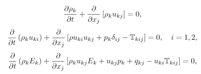
Solving these equations with a pen and paper is possible only in a few, relatively simple situations. In most situations, we therefore use numerical fluid mechanics (CFD – computational fluid dynamics), in which computers are used to find the solutions to the equations instead.
The author of this blog post, Knut Emil Ringstad, is studying for a PhD at NTNU through the HighEFF research centre, which carries out research on energy efficiency in Norwegian industry. You can find out more information on the work of HighEFF by subscribing to the newsletter.
Basic principles of numerical fluid mechanics
We will use a simple analogy to explain CFD and how you can use it as a tool. Imagine CFD as a board game with playing pieces, a game board and a set of rules.

Let’s start with an easy example. You have a square game board that you fill with arrows. The game board represents the area in which you want to investigate flow and each square constitutes a small part of the area. The arrows represent the speed of the fluid in the square. You then add a black playing piece symbolising a volume containing some quantity. The quantity will typically be mass (density), temperature or momentum.
First, we introduce two simple rules:
- One round equates to one step forward in time (a time step) and all pieces must be moved.
- The pieces must be moved in accordance with the arrows (speed) in the square the piece is in.
We can play a round using these rules. The simple animation below shows you how a round can look:

Until now, the arrows have been placed arbitrarily on the board. To work out how the arrows should be placed, we must solve the momentum equations. Momentum and speed belong together in the ratio: momentum = mass * speed.
In our analogy, this corresponds to playing using the arrows as playing pieces. In other words, the black piece is an arrow (corresponding to speed or momentum). When we play using the arrow as a piece, we also need to take into account its effects on the board in rule 2, i.e. that the pieces must be moved in accordance with the arrows (speed) in the square it is in. This is illustrated here:

We are going to try to add another rule so that you have a decent toolbox before you try it out on an actual problem. We refer to rule 3 as the law of diffusion. This says that if the difference between two neighbouring squares is two or more, move one piece from the square with the highest value to the square with the lowest value.
This rule is best explained in the context of momentum. Here, the law of diffusion corresponds to friction between different layers of flow, illustrated in the animation below. Here, you first have a flow with a high speed at the top and a flow with a lower speed below. The friction between these layers accelerates the fluid at the bottom and decelerates the fluid at the top.

A practical example of CFD
Using the three rules and the playing pieces, we can now try a simple problem. Imagine a large tank of water, for example, and an outlet pipe at the bottom. We want to find out what happens to the pattern of flow in the pipe when it is opened.
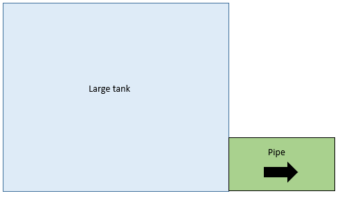
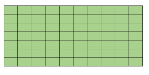
We first have to identify the area and create a game board. In CFD, this is referred to as constructing a mesh.
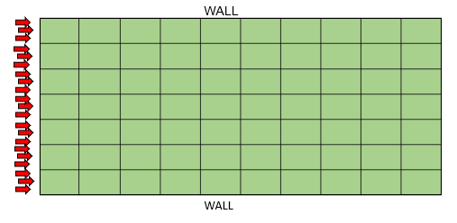
We then choose what should happen along the boundaries on the outside of the mesh. Here, we specify that the inlet speed of the fluid is high (see image below) and that the speed must be equal to zero along the walls.
When we start the game using rules 1-3 for the arrows, we end up with a course of events similar to the figure below.
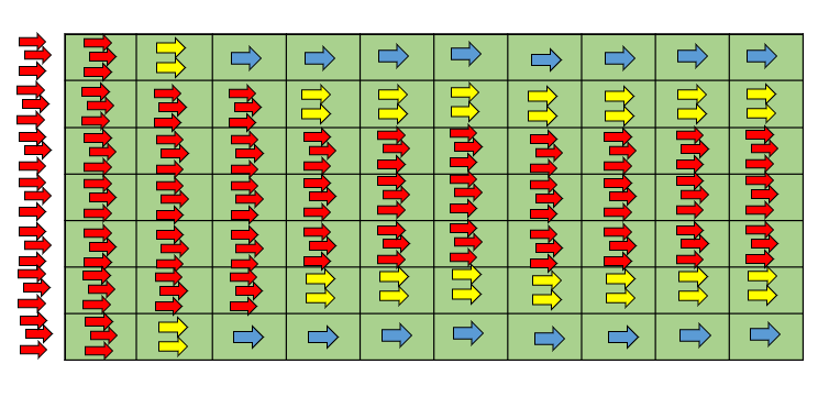
The speed of flow along the wall declines and we get a high-speed core in the middle of the pipe. In fluid mechanics, this is called entrance length, see figure below.
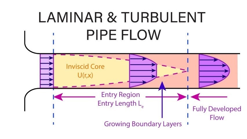
This is a simplification of how to solve CFD problems, but provides good intuitive understanding of fluid flows. In reality, the speed would be specified with more arrows for higher accuracy. In the above example, an arrow could correspond to a speed of e.g. 0.1 m/s. However, the use of decimal figures is preferred for simulations.
We find the answers to the equations at the top of this blog post when we play the board game. Even though the equations look complicated, we can find our three rules in a simplified form of equation 2:

This rendition of the equation constantly repeats in fluid mechanics, as these three effects (changes in time, advection, diffusion) are fundamental in flow transportation. To add additional effects such as gravity or pressure, we must also add more rules. Using these rules of play, you can create a large range of simulations.
Later on in this blog post, I will touch on more advanced subjects.
Mesh design
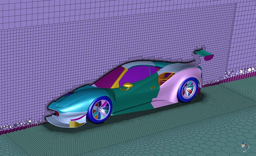
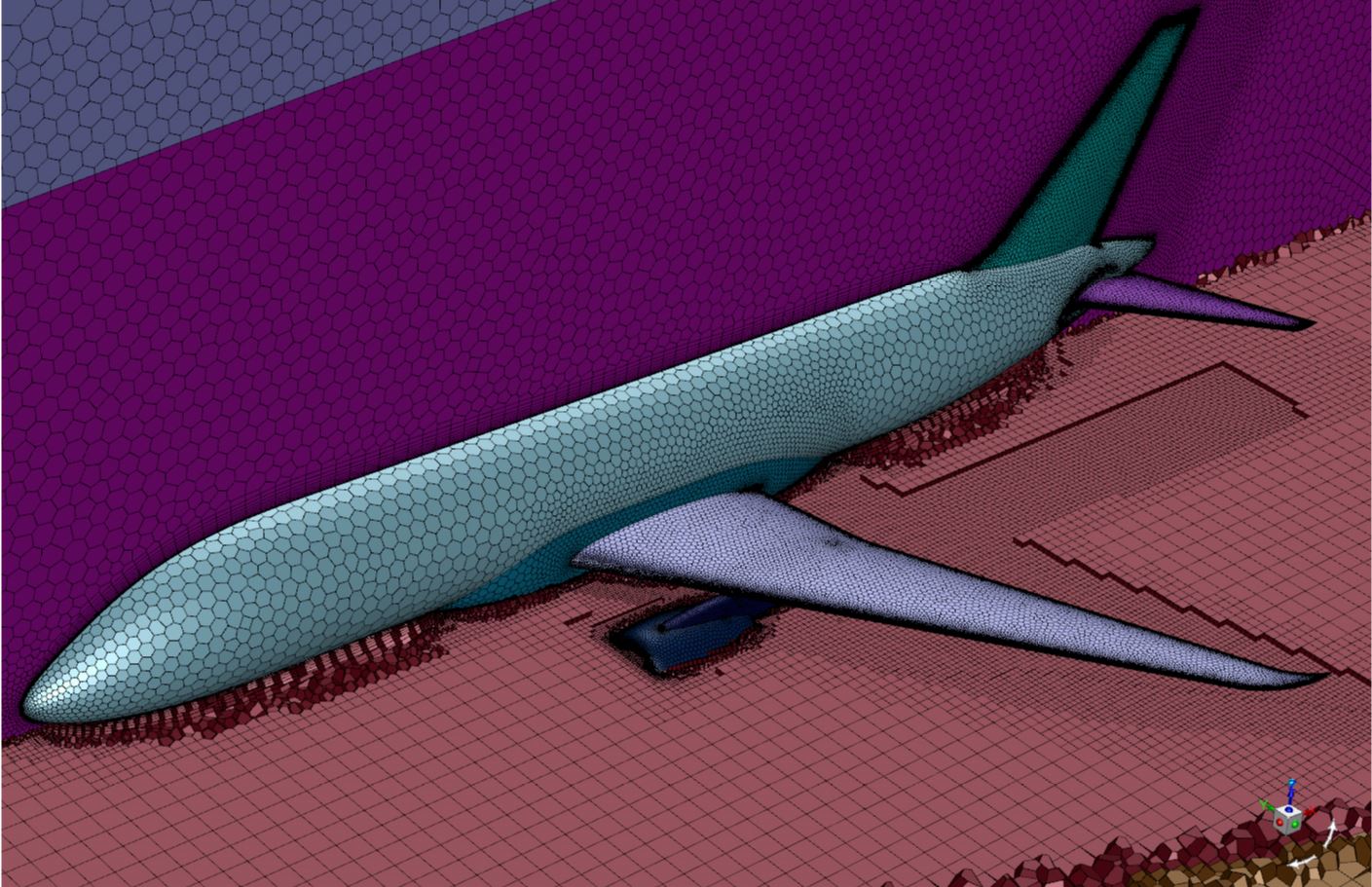
So far, we have only used square game boards (mesh) in which all squares are of equal size. In real simulations, you would adapt how the squares are configured to capture as much detail as possible using minimal computing power. In some simulations, millions of squares must be used, which takes up lots of storage space on your computer and also takes several weeks to calculate.
A better mesh will reduce the calculation time, make the simulations more stable and cause fewer errors. In an industrial context, a lot of time is therefore invested in advanced mesh design. You can see two examples of advanced mesh design below.

Turbulence
Turbulence may occur when the speed of flow increases. Turbulence is a pattern of flow in which structures occur which break themselves down into smaller and smaller pieces. These structures can be simulated in the same way as discussed in our analogy.

The problem is that these structures eventually become so small that enormous amounts of computing power will be required. We therefore prefer to introduce turbulence models that attempt to mimic the effects of having many small turbulent structures in the flow. The most famous of these models are the k-epsilon and k-omega models. Even though these are advanced models, you can recognize the same rules we used in our analogy:

Applications
CFD is a versatile tool that can be used to solve a broad range of problems. CFD can, for example, help you with:
- Gaining a deeper understanding of flow. – Detailed descriptions of physical processes.
- Designing new or improved components and equipment.
- Creating improved models for system scale tools.
- Optimising components.
- Creating digital twins of real products.
In conclusion, I would like to note that it is important to be critical when a CFD model is presented. Results can be misleading if the work has not been executed well. Some points to look out for when assessing a CFD model:
- Has a mesh study been conducted?
- Have different models been subject to critical assessment and, preferably also, comparison?
- Have the model results been compared against an actual experiment?
Other very interesting topics that have not been covered here include:




Comments
No comments yet. Be the first to comment!