Model testing has been, and still is, the dominant method to predict the propulsion performance of ships. However, the use of Computational Fluid Dynamics (CFD) methods for the same purpose is becoming increasingly common and is also becoming an integral part of the ship design process.

The greatest advantage of CFD is the possibility to directly perform predictions at full scale, thereby reducing uncertainties related to the influence of Reynolds number (known as scale effect). They can be conducted in a time- and cost-effective manner, especially when best practices are established and automated templates are developed. Even though the International Towing Tank Conference (ITTC) has been developing and updating recommended procedures and guidelines since 2011, the predictions using CFD can have significant variation between each user.

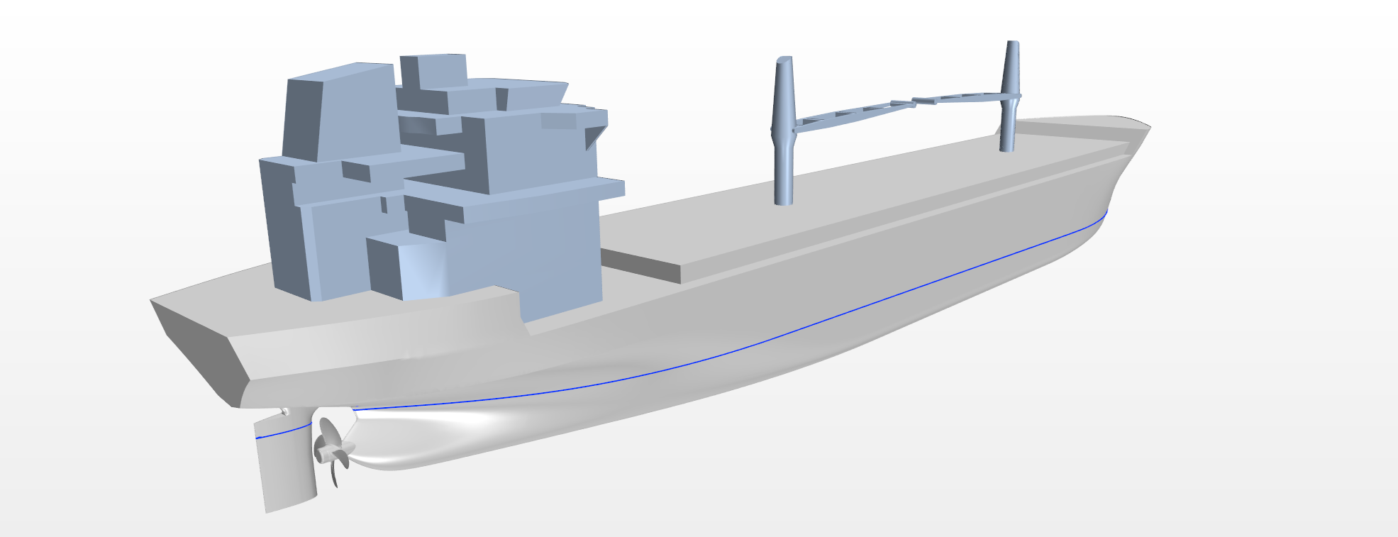
Recently, SINTEF Ocean participated in the ongoing Joint Research (JoRes)[1] project where prediction of full-scale ship performance using CFD of the benchmark vessel MV REGAL was performed. Comparisons were made of both model test and sea trial data for propeller open water characteristics, calm water hull resistance and ship self-propulsion. This was a blind exercise where participants of the project employed their best practices and gained access to the benchmark data after submitting their results.

SINTEF Ocean used this opportunity to validate our CFD templates and further investigate how surface roughness and turbulence models impact the ship predictions. Our findings were published in the seventh International Symposium on Marine Propulsors (smp’22)[2] and in Journal of Marine Science and Engineering (JMSE)[3].

Propeller open water

The propeller open water simulations were performed in full-scale using the same propeller setup as in self-propulsion conditions. This means that the propeller was operating in pushing mode behind the ship hull, unlike the conventional open water model test setup of pulling mode that was used as benchmark data.

For this exercise we investigated different surface roughness treatments (smooth and roughness height of 8.68 μm and 30 μm) and turbulence models (conventional RANS and higher fidelity DES, LES and SRH). Note that the roughness height employed corresponds to equivalent sand-grain roughness height and not actual measured roughness height. Surface roughness was not investigated for LES and SRH as these models are not compatible with roughness treatments in the employed CFD software. The results for smooth surfaces are shown in Figure 2 and rough surfaces in Figure 3.

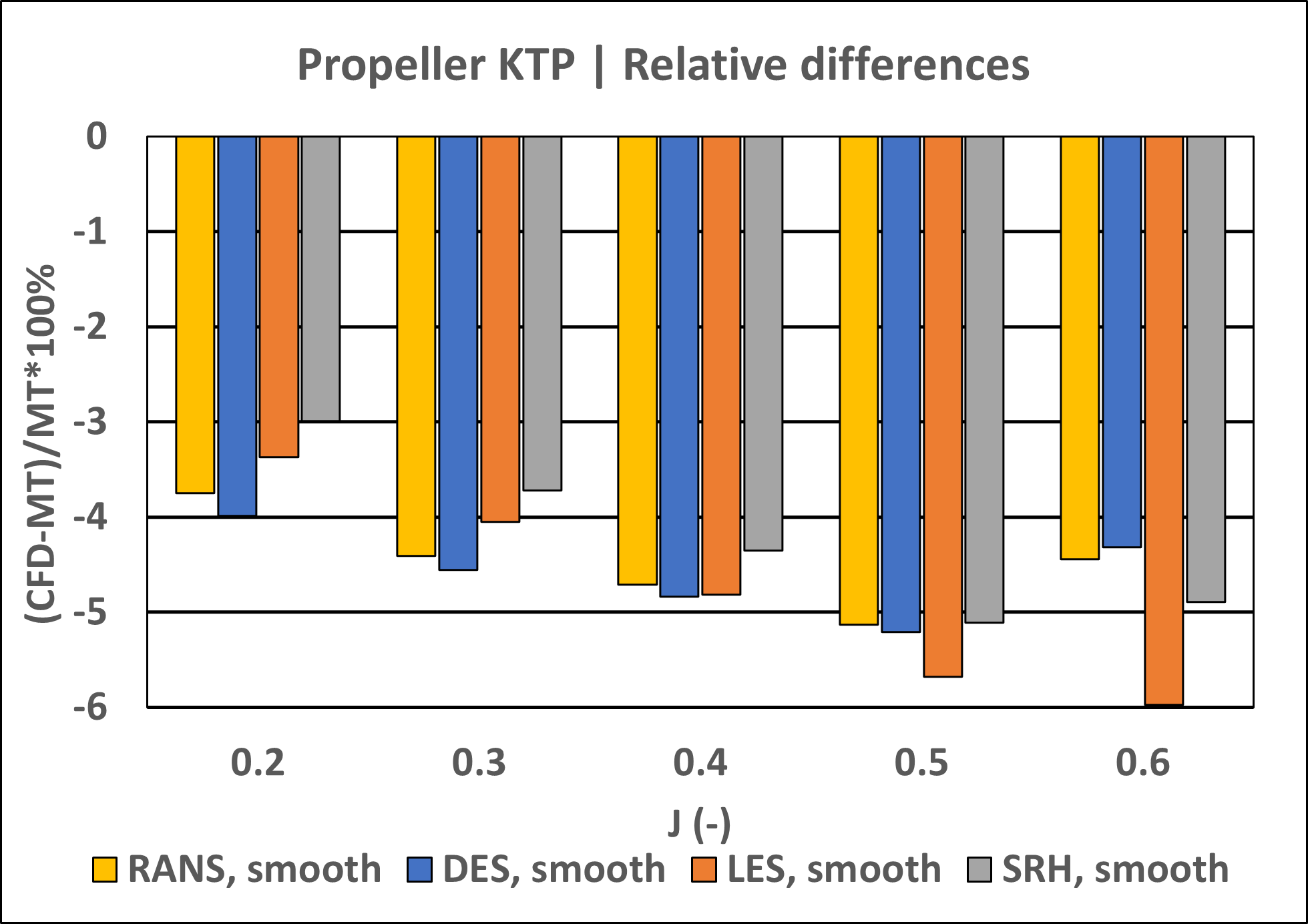
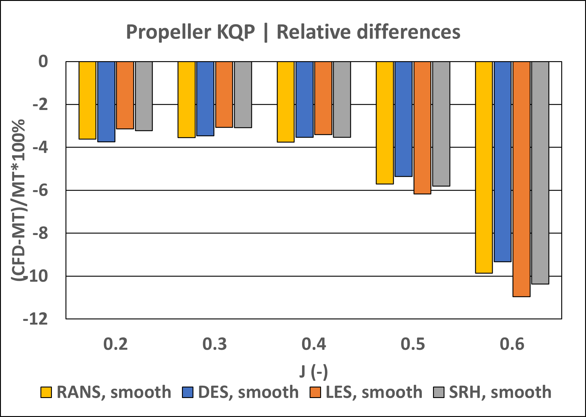
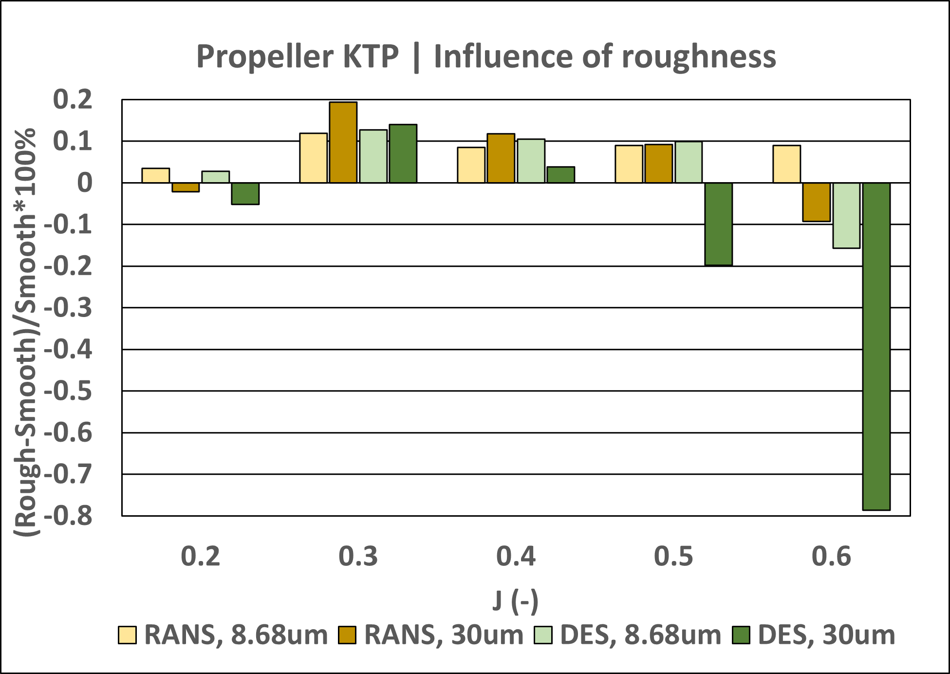
Figure 2: Comparisons between computed and measured propeller thrust, torque and efficiency.

In the range of advance coefficient (J) 0.2-0.5 there is a difference of 4-5% compared to model tests for both thrust and torque. This offset is mainly explained by the different shaft arrangement and hub caps utilised between CFD and model tests. At J = 0.6, influence of Reynolds number becomes more prominent explaining the larger difference for torque and hence efficiency.

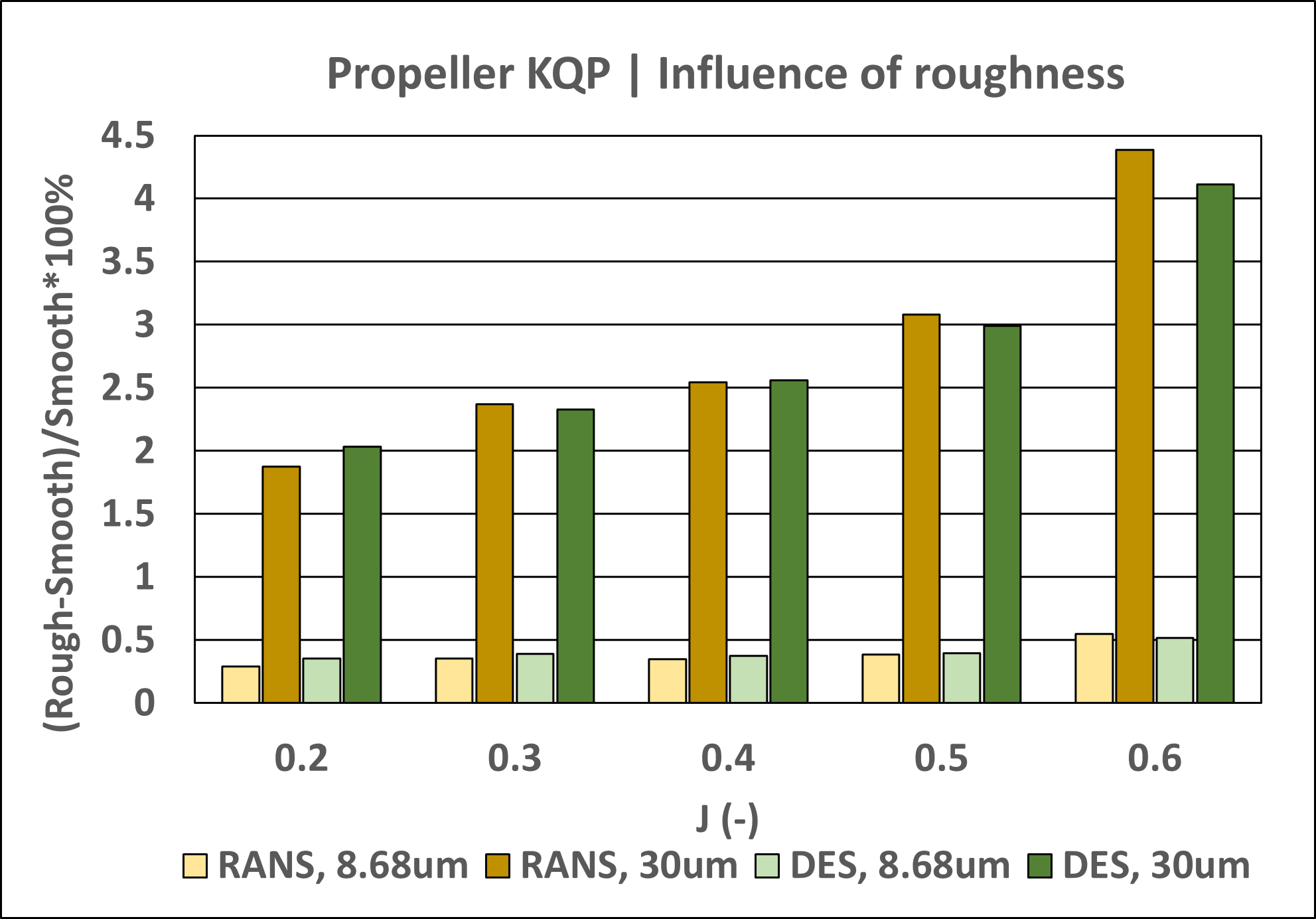
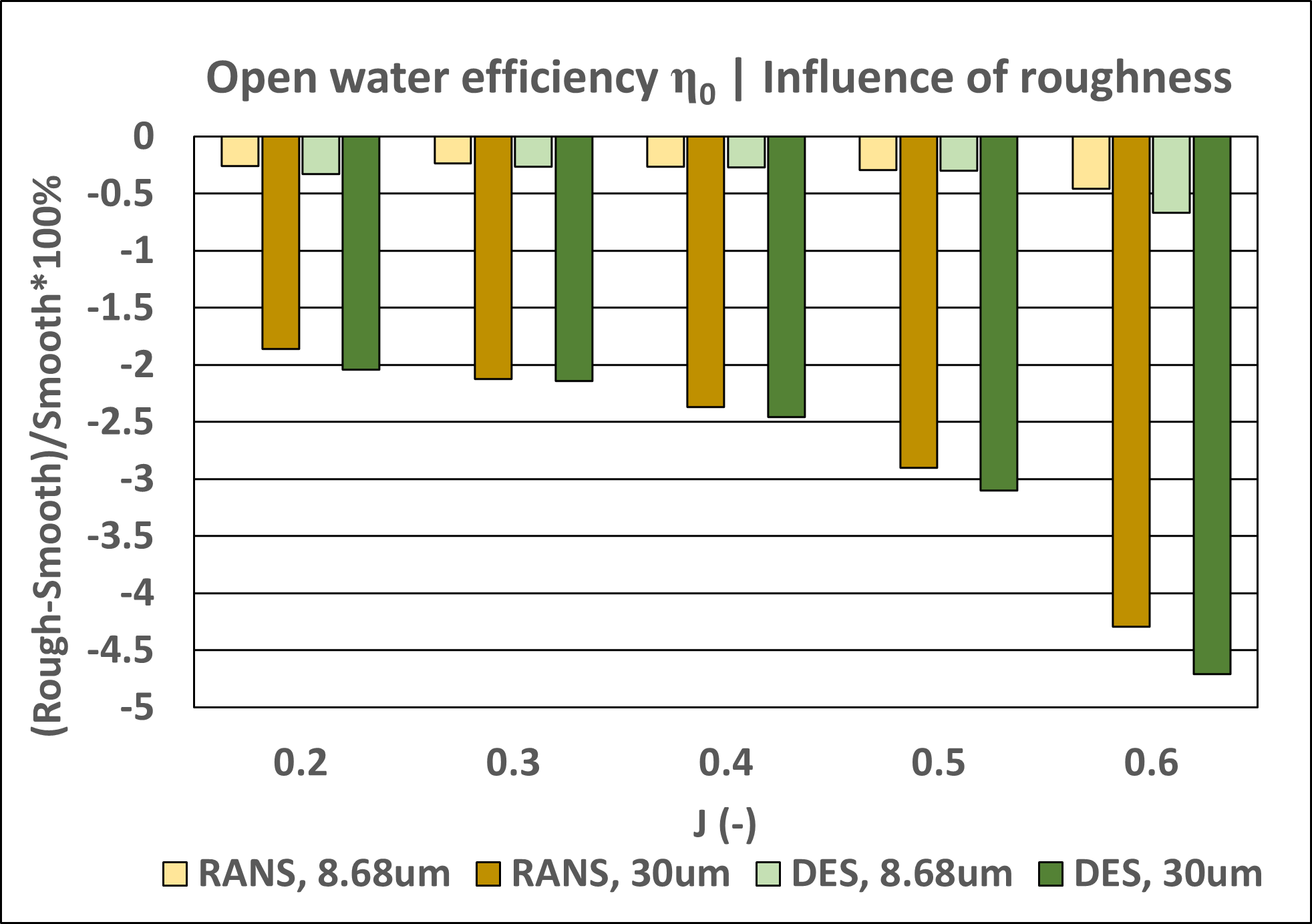
Figure 3: Influence of surface roughness on propeller thrust, torque and efficiency.

Both RANS and DES turbulence models predict similar magnitudes of the roughness effect, which is mainly seen in the increase of propeller torque and, consequently, the decrease of propeller efficiency. These influences become more significant at higher J values, where the relative contribution of the frictional component is greater.

The main difference between the turbulence models is, however, not in the propeller characteristics, but rather in the vortical structures in the slipstream generated by the propeller, as shown in Figure 4. While the vortical structures may not be of high importance in open water configuration, they play an important role when interacting with appendices, such as rudder, located downstream of the propeller.

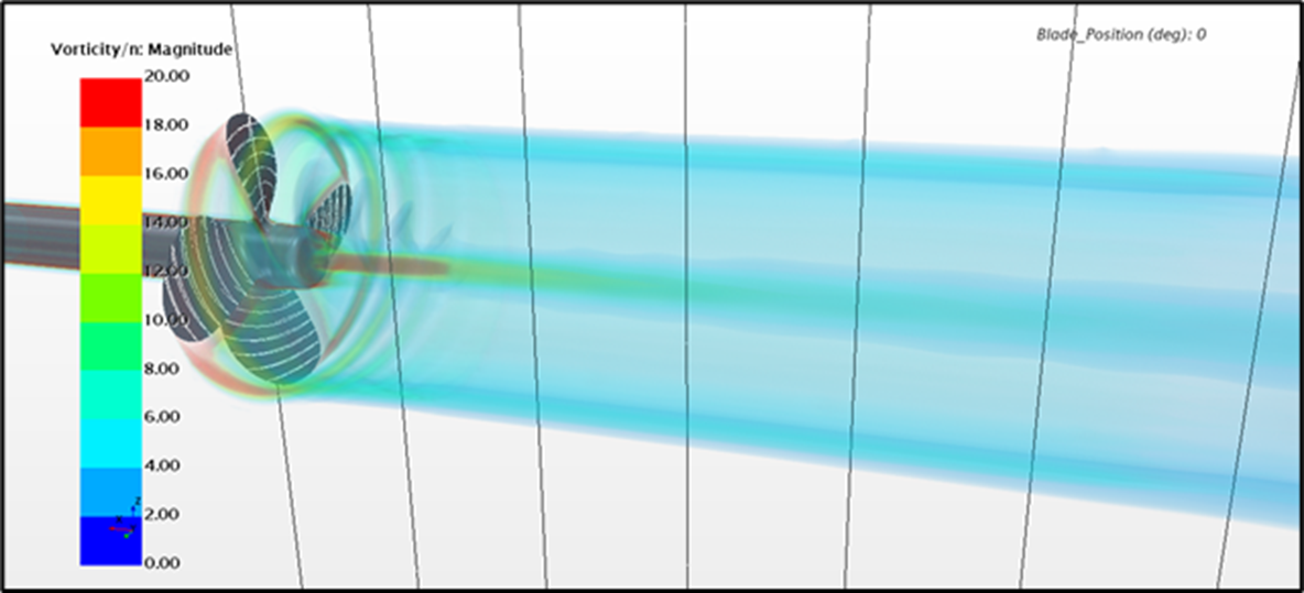
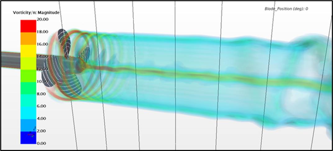
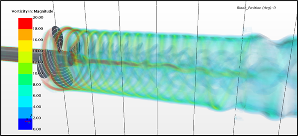
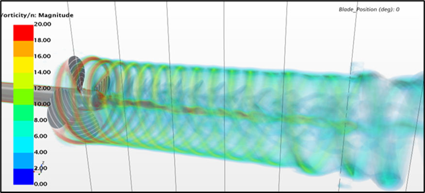
Figure 4: Vorticity magnitude in propeller slipstream. From top to bottom: RANS, DES, LES, SRH.

Calm water resistance

For the resistance simulations we wanted to focus on various surface roughness heights. Through preliminary studies, 80 μm equivalent sand-grain roughness height was selected as the most appropriate modelling of the old, but cleaned, hull and rudder of MV REGAL, run with both RANS and DES. In addition to the 80 μm, smooth and 150 μm roughness height using RANS was also run to give further insight in how roughness affects the resistance. Results can be viewed in Figure 5 with CFD results compared to model test prediction.

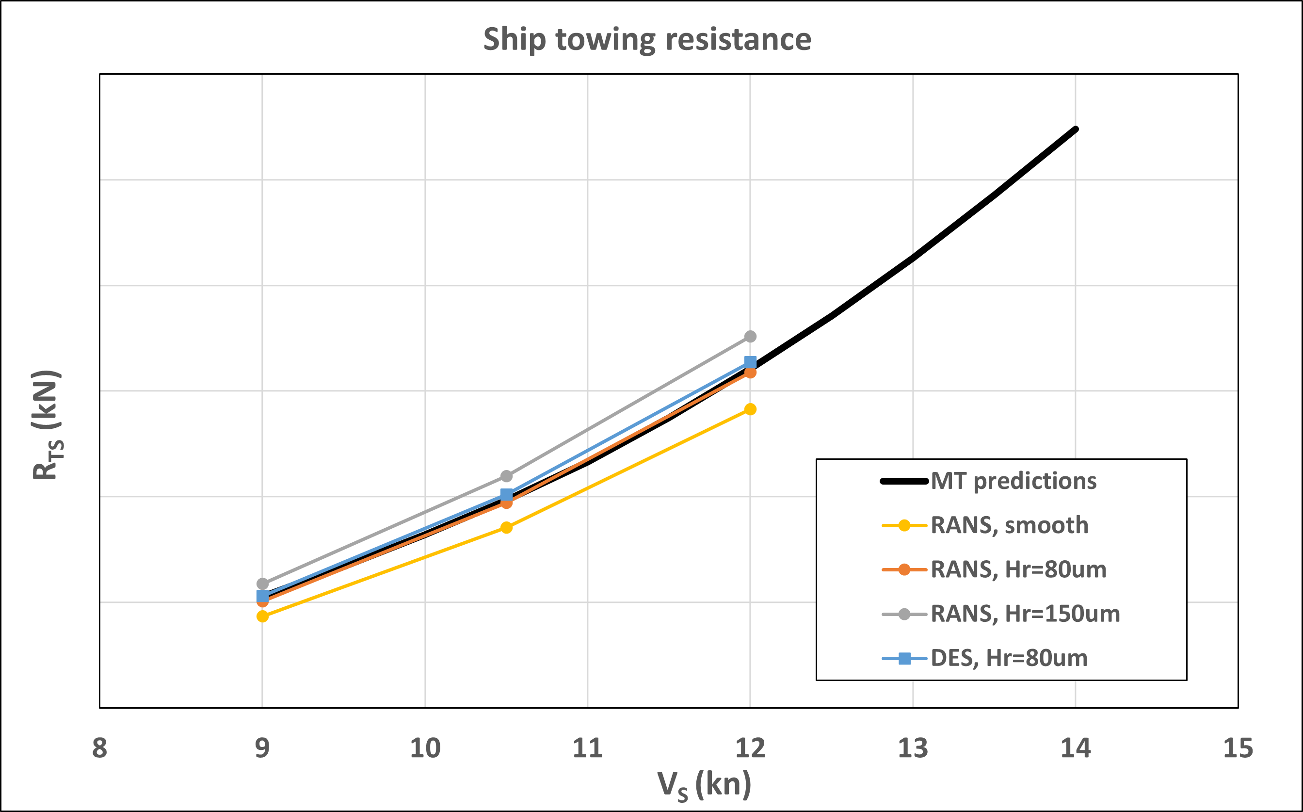
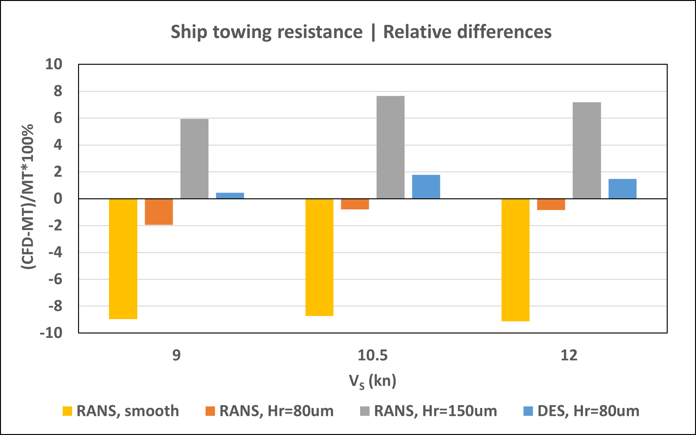
Figure 5: Full-scale ship resistance by CFD and predicted from model tests.

Both RANS and DES with roughness height of 80 μm are within 1-2% of the model test prediction. Smooth surface underpredicts with 9% and the 150 μm case overpredicts by 6-8%. While the surface roughness modelling is of higher significance for hull resistance, the choice of turbulence modelling has a far more noticeable impact on the depiction of nominal wake on the propeller plane, as shown in Figure 6 with time-averaged nominal wake of RANS and DES.

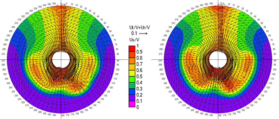
As expected, the DES solution results in a heavier wake field (nominal wake fraction 0.518 compared to 0.495 predicted by RANS) with better-resolved separation areas on the portside, starboard, and below the stern tube. However, it is in the time-varying wake field where the differences are most prominent. While the wake field in the RANS method hardly shows any changes with time, the wake field resulting from the DES simulation is highly unsteady. The separation zones downstream of the shaft tube contain a collection of eddies with varying sizes and intensities. These eddies continuously interact, causing the shape and extent of the separation zones to change over time. To illustrate this, Figure 7 presents instantaneous snapshots of the wake field from the DES simulation taken with a time interval of 5 s.

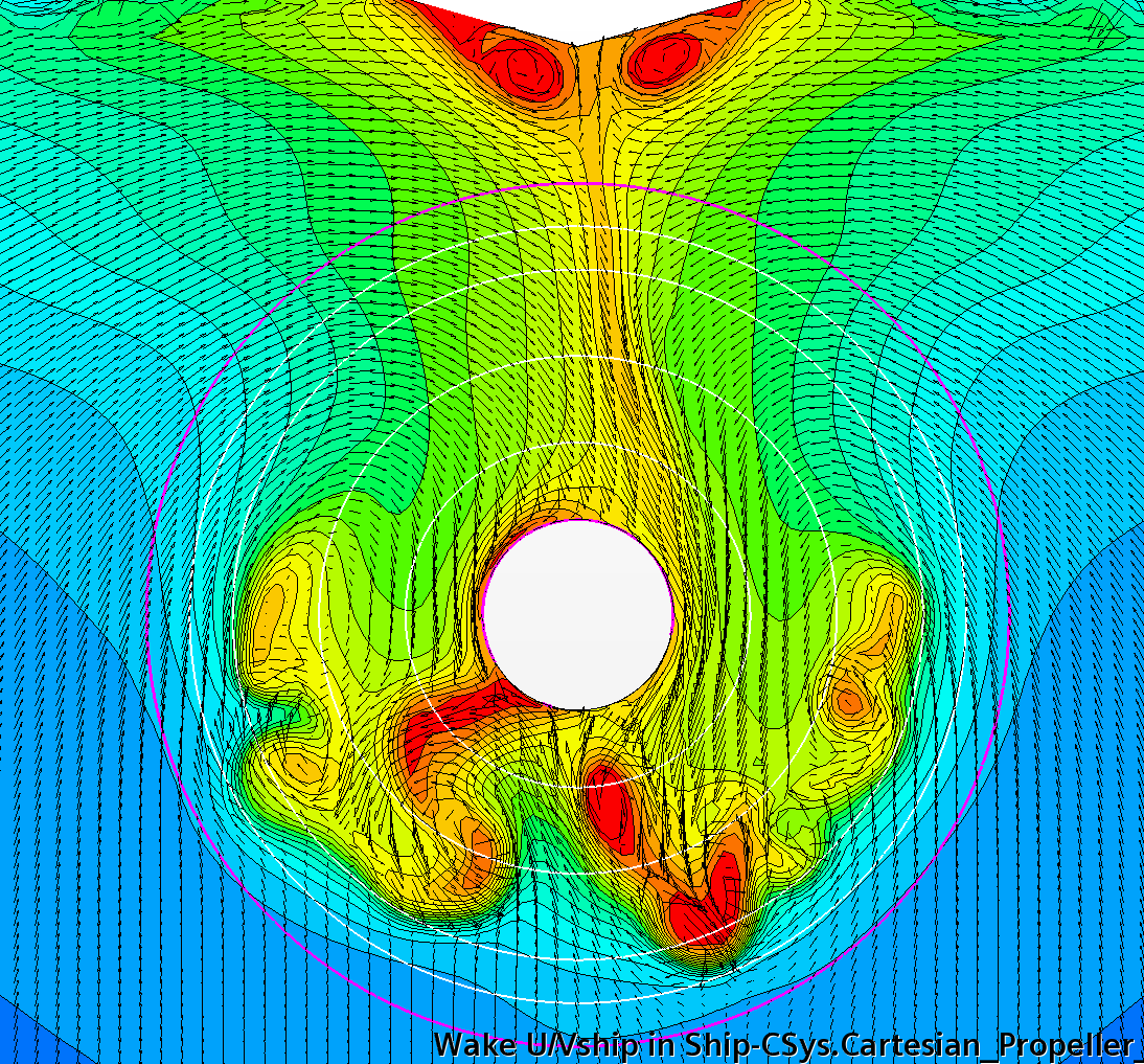
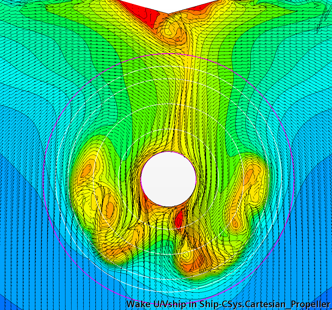
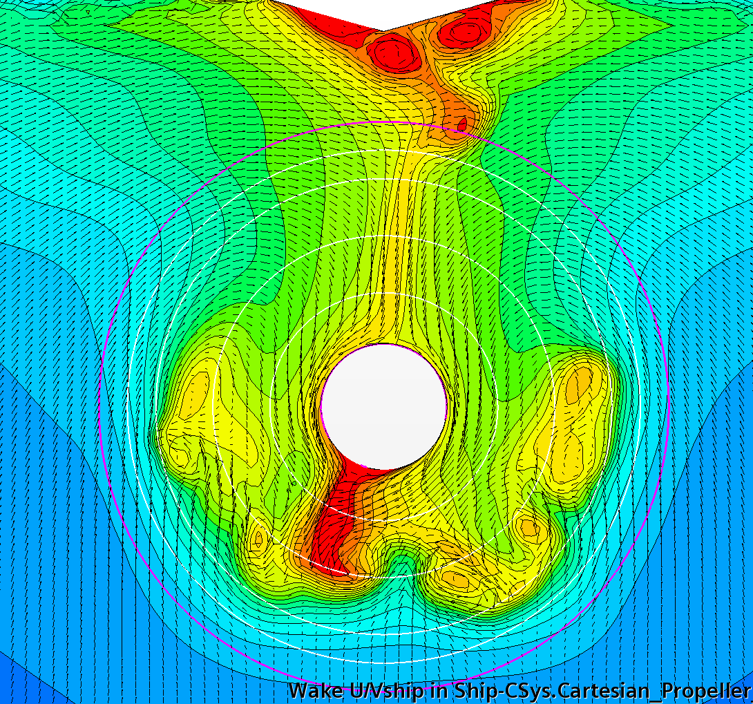
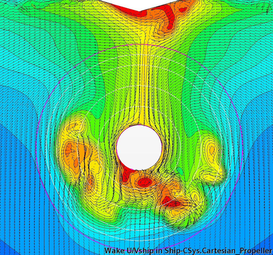
Figure 7: Instantaneous snapshots of the nominal wake field from DES. Time interval 5 s.

Self-propulsion

The self-propulsion simulations are based on the resistance simulations including the propeller. The propeller RPM is adjusted until self-propulsion point is reached. These simulations were performed with surface roughness of 30 μm on the propeller and 80 μm on hull and rudder for both RANS and DES. An additional run with RANS and 150 μm on hull was also conducted to see how it impacts the self-propulsion results. The numerical results, compared to both model tests and sea trials are shown in Figures 8-10.

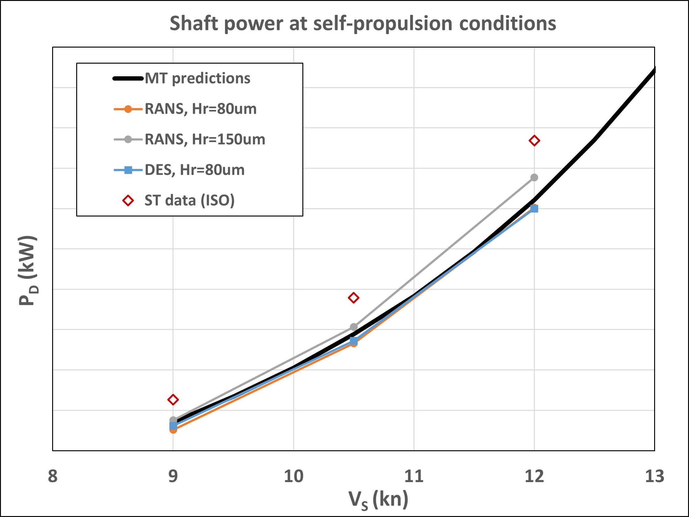
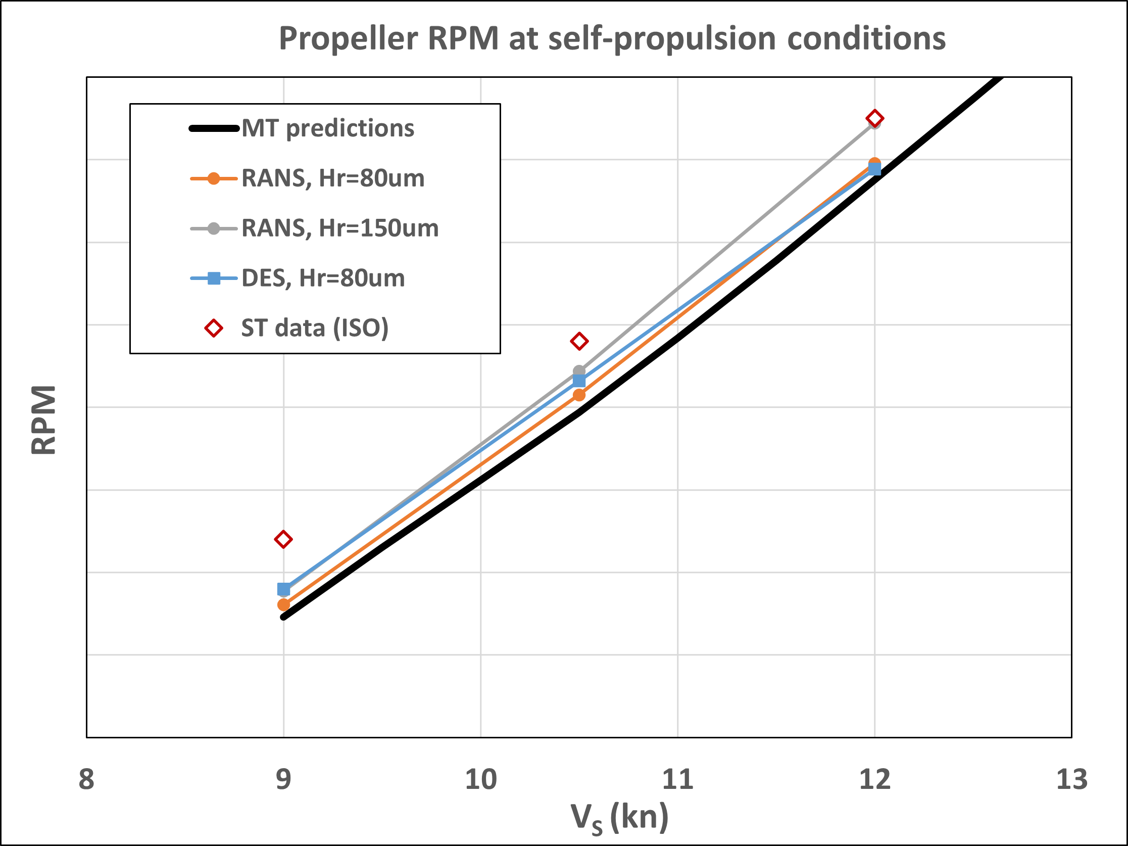
Figure 8: Comparison of propeller shaft delivered power (left) and RPM (right) at self-propulsion point.

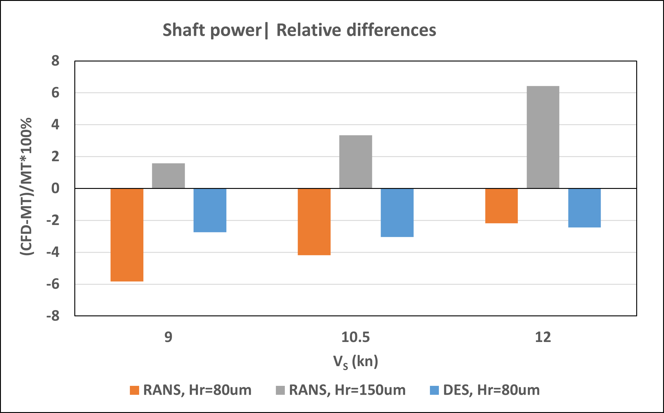
Figure 9: Relative differences between CFD and model test prediction.

It can be concluded that both the RANS and DES methods provide comparable prognoses of the ship’s propulsion performance when using a hull roughness of 80 μm, which is close to the predictions derived from model test data. The DES results are somewhat closer to model test predictions for shaft power and RPM, with relative differences of approximately 2.5% at all ship speeds. The RANS results are closer to model test data in terms of RPM (approximately 1%), but they reveal larger deviations in shaft power (2–6% depending on speed).

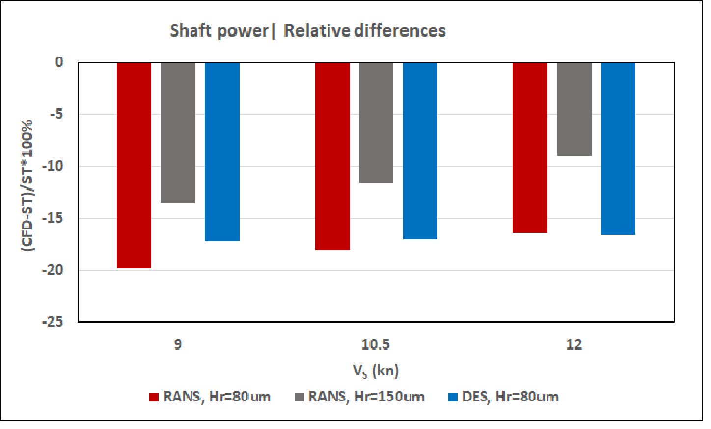
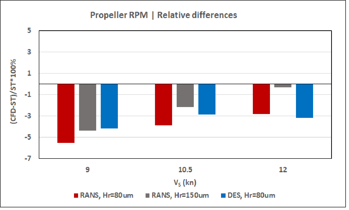
Figure 10: Relative differences between CFD and sea trial data

Both the CFD calculations and model test predictions underestimate shaft power and RPM compared to the sea trials data post-processed according to the ISO15016 standard. For the CFD results using the DES method and a hull roughness of 80 μm, the underpredictions amount to 3–4% in terms of RPM and 17% in terms of shaft power. The RANS calculations performed with the increased value of hull surface roughness of 150 μm reduce these differences to approximately 2% and 12%, respectively.

The high values of hull surface roughness and numerous surface imperfections documented on MV REGAL in the JoRes project indicate that the hull surface conditions may indeed be one of the factors explaining the deviations between the predictions and sea trials. However, an even more likely reason is related to the presence of bilge keels on the ship hull and sacrificial anodes on both the hull and rudder, which were not considered in the CFD simulations and model test predictions. The combined contribution of these constructive features can easily amount to 11–13% of increased hull resistance in propulsion conditions. This increase may be even higher in the case of bilge keel misalignment. When combined with the surface conditions of a 25-year-old ship hull, these influences may result in an increased power demand of 15%. Therefore, the differences between the performance predictions and sea trials data found in the present case are not at all surprising and even quite expected.

Conclusion

For full-scale ship performance predictions, the comparative results demonstrates that the applied CFD modelling practices are mature and capable of predicting a ship’s performance characteristics with the accuracy required for practical applications. In particular, the results of the DES method applied in these analyses are found to be in good agreement with the prognosis based on model tests. In this case, the differences in terms of shaft delivered power and propeller RPM do not exceed 2.5%, which is well within the accepted range of CFD/EFD calibration factor (0.95 to 1.05), according to IACS Guidelines[4]. The DES method provides a good compromise between the computational demand, accuracy of prediction of propeller and hull forces, and resolution of flow details. It also supports the inclusion of surface roughness and shows little sensitivity to the simulation time step.

Both CFD calculations and model test prognosis underpredict shaft delivered power by 12-17% and propeller RPM by 2-4%, depending on the applied value of equivalent sand-grain roughness height, when compared to sea trials data. As mentioned, these differences are thought to be caused by additional components not included in either CFD or model tests, as well as the surface condition of the ship’s hull. The use of accurately scanned hull, propeller, and rudder geometries is therefore deemed highly important for direct comparisons between full-scale CFD predictions and sea trial data on old ships in service.

More results, discussion and model setup used in this work can be viewed in our publications [2], [3].

[1] https://jores.net/

[2] https://www.marinepropulsors.com/proceedings/2022/1-1-2.pdf

[3] https://doi.org/10.3390/jmse11071342

[4] IACS Guidelines on Numerical Calculations for the Purpose of Deriving the Vref in the Framework of the EEXI Regulation. No.173, 10 November 2022.