By predicting how various real-world phenomena will play out, we can take educated actions to mitigate the negative consequences, leading to a healthier ocean.
Throughout history, people have searched for meaning in random events. Fortune tellers have attempted to use cards in random order, tea leaves, and even the intestines of animals as a guide to the future. Gamblers have tried to predict seemingly unpredictable events, such as dice rolls or the results at the roulette wheel.
However, random numbers can also be used to make models of physical phenomena, and these can be used to predict outcomes of experiments with excellent accuracy. Here, I will briefly describe a few points from the history of random numbers in the physical sciences, and give some examples of current uses.
From science to finance
In 1827, the Scottish botanist Robert Brown published a description of what is now known as Brownian motion. He used a microscope to observe small particles suspended in water and found that they were perpetually in a state of random, jittery motion.
In 1905, Einstein published a now famous paper where he described these motions in terms of the theory of atoms. His idea was that Brownian motion was caused by random collisions between the molecules of the liquid, and he pointed out that careful observations of Brownian motion in a microscope could actually allow us to calculate the mass of those molecules.
Einstein’s paper, along with observations by Perrin (1909), became one of the key pieces of evidence that led to widespread acceptance of the existence of atoms. Around the same time, Langevin (1908) wrote down an equation describing Brownian motions in terms of a random force. This type of equation is now called a stochastic differential equation (SDE) and is used for many purposes in both the physical sciences and in finance.
Carefully-calculated averages
The collisions between molecules and particles, that are the cause of Brownian motion, are not truly random. They follow well-known physical laws and can in principle be predicted. However, the enormous number of molecules in even a single teaspoonful of liquid means that it is practically impossible to make exact predictions of their motion. (In fact, it might even be theoretically impossible, due to the finite precision of computers.)
Hence, their motion appears random to us, and we cannot make exact predictions of the Brownian motion of a single particle. However, we can easily make predictions about the average behaviour of a collection of particles, and this is often just as useful. The key point is that we do not need to know the true motions of the atoms and molecules to make these predictions, we only need to be able to produce random numbers with the same distribution.
As a more familiar example, let us say we would like to find the average height of the population in Norway. The definition of an average is simple. You just add up the heights of all the people in Norway and divide by the number of people. However, in practice, asking 5 million people how tall they are is not so convenient. Instead, we can ask a sample of 1000 people, randomly selected in such a way that they are representative of the population, and calculate the average of those 1000. This procedure is likely to give us a quite good estimate of the average height of the whole Norwegian population.
Minimising the margin of error
And in fact, a very useful theorem called the Central Limit Theorem, can tell us how good our estimate is likely to be. It tells us that the error in our estimate will go down if we include more people in our sample, and specifically that the error goes down proportional to 1 divided by the square root of the sample size. This is similar to how public opinion pollsters calculate the margins of error in, for example, polls of voters ahead of elections.
The use of random numbers in computational physics has a history that is as old as computers themselves. One of the first uses of ENIAC, the first general purpose digital computer, was to calculate how neutrons behave inside a nuclear weapon, by use of random numbers.
The method was named the Monte Carlo method, after Stanislaw Ulam’s uncle, who would borrow money from relatives and go to Monte Carlo to play in the casino (Metropolis, 1987). Nowadays, the term “Monte Carlo method” is often used more generally to refer to schemes where repeated sampling of random numbers is used to compute the expected outcome of some physical process.

Applying random numbers to ocean science
An example of how random numbers and Monte Carlo methods are used in our activities at SINTEF Ocean, is our work on the transport of pollutants in the ocean. We know that for example oil or plastics that float on the surface of the ocean are transported by the wind and the ocean currents.
The large-scale patterns of the wind and the currents can be predicted reasonably well. We know for example that the weather forecast is generally quite accurate for the next few days. However, our forecasts for the wind and the current cannot predict what will happen in detail. The weather forecast might for example say that there will be on average 10 m/s wind towards the north-west, and up to 15 m/s in the gusts, but it cannot predict when each gust arrives, or how strong it will be.
Similarly, for the ocean currents, we know that the current generally moves north along the coast, and we can predict the tides with great accuracy, but there is a lot more going on in the ocean. Everywhere, there are smaller and larger “eddies” that cause the path of the water to twist and turn. We know the equations that describe these motions, so they are in principle predictable, but in practice the amount of data needed to describe the entire ocean is far too great for us to handle.
Predicting pollution patterns for a healthier ocean
To take these unpredictable details into account in a model for pollution that floats on the sea surface, we use the predicted wind and current as a guide. Then we add random displacements to account for the small-scale motion, which is not represented in the predictions. On the computer, our models can calculate the trajectories of hundreds of thousands of floating particles, all experiencing different versions of the random motion. Together, these particles give us a prediction of how the pollution will move and spread out across the ocean.
In the case of an oil spill at sea, for example, we can use these models to predict how the oil will move over the next days, and use this information to direct efforts to collect the oil. We can also use models to analyse what might happen in a hypothetical oil spill. Such an exercise will always have uncertainty, but with Monte Carlo methods we can predict a range of possible outcomes, and describe both the most likely outcomes, as well as the “worst case scenarios” that are less likely, but still possible (Nordam, 2017).
A direct contribution to Life Below Water
Plastics in the ocean is also an important, and increasingly visible environmental problem. This is a problem of a chronic nature, since plastics are continuously added to the ocean from widely distributed sources. We can use models to study long-term transport patterns and identify areas where the plastics will collect. Models can also be used to study the problem in reverse: Given observations of where plastics are found, we can calculate the most likely source-areas (Strand, 2021).
An important strength of models is that they can be used to “fill in the gaps” between observations. We will never have as many observations as we would wish, especially in the open ocean away from the coast, where it is expensive and time consuming to take samples and make observations. By combining models and observations, we can try to describe the situation in the ocean as a whole. Using models to both describe and predict the fate of pollutants in the ocean helps us make informed decisions about how best to act, and is an integral part of how we at SINTEF Ocean contribute to the UN Sustainable Development Goal 14: Life below water.
References:
Einstein, A. (1905), “On the movement of small particles suspended in stationary liquids required by the molecular-kinetic theory of heat” (translated from German), https://einsteinpapers.press.princeton.edu/vol2-trans/137
Langevin, P. (1908), “On the theory of Brownian motion” (translated from French), https://aapt.scitation.org/doi/10.1119/1.18725
Metropolis, N. (1987), “The Beginning of the Monte Carlo Method”, https://permalink.lanl.gov/object/tr?what=info:lanl-repo/lareport/LA-UR-88-9067
Nordam, T. et al. (2017), “Impact of climate change and seasonal trends on the fate of Arctic oil spills”, https://link.springer.com/article/10.1007/s13280-017-0961-3
Perrin, J. (1909), “Brownian movement and molecular reality” (translated from French), http://web.mit.edu/swangroup/footer/perrin_bm.pdf
Strand, K. et al. (2021), “Potential sources of marine plastics from survey beaches in the Arctic and Northeast Atlantic”, https://www.sciencedirect.com/science/article/pii/S0048969721030801


Comments
No comments yet. Be the first to comment!