Over the next seven years, international shipping must reduce its total emissions by 20 to 30 percent (IMO)1. To achieve these goals, it’s more important than ever to understand what is driving emissions from today’s fleet. Then, we’ll be able to implement efficiency measures while developing zero emission solutions.
Shouldn’t we just start measuring then? Modern ships are full of sensors, but that doesn’t automatically mean that the data has been logged or is easily accessible. If systematic measurements were to be initiated, it would in most cases entail the considerable job of installing a logging system. Since we know that the average age of Norwegian-owned vessels in short sea shipping is 20 years2, it is also reasonable to assume that many vessels will require extensive instrumentation improvements. Another aspect is that the weather can significantly affect a ship’s energy consumption. Therefore, when taking systematic measurements over shorter periods of time, there will always be uncertainty as to how representative the collected data are in relation to the ship’s operations over a longer period of time – and it’s the total consumption over longer periods of time that counts when trying to achieve the IMO targets.
It may seem like an insurmountable task to estimate the annual consumption of one or more vessels, but there are ways to solve this. In order to understand one of the methods, we must go from the wet element to one of the driest places on earth – namely, the Nevada desert. During World War II, the United States tested atomic bombs there. One of the researchers in the Manhattan Project was named Enrico Fermi. He reportedly observed the movement of small pieces of paper during the nuclear explosion test and used this information, along with some mental arithmetic, to estimate the strength of the explosion. A few weeks later, his estimate was confirmed through the analysis of the data from the advanced instruments used during the test3. By using his domain knowledge combined with inaccurate data, Fermi was, in other words, able to arrive at almost exactly the same answers as very sophisticated measuring instruments. The example is perhaps most suitable for confirming what one might have already suspected: Fermi knew his stuff. At this point in time, the man already had the Nobel Prize in Physics standing on his mantlepiece. While Fermi’s estimate is undoubtedly impressive, can this clever method also be applied in practice and used in other contexts? For example, to tell us something about the energy consumption of Norwegian ships? Yes, because it is basically about the same thing: providing good (enough) estimates based on the information available.
The key to Fermi’s approach (often called Fermi estimates) is to break down large, almost insurmountable problems into a series of smaller tasks, for which, in isolation, one may be able to provide fairly reasonable estimates. In addition to the fact that the breaking down itself is useful for solving a problem, it has also been shown time and time again that the total estimates are surprisingly accurate.
From Trinity to ships3: Fermi estimates of energy consumption. Fermi estimates really come into their own in situations where it is difficult to access sufficient amounts of measurement data. An example of such a situation is the energy consumption of sailing ships. A shipping company can get an overview of the cost of fuel, but bunkering doesn’t take place very often. As a result, fuel receipts will not document the short-term variations in energy consumption, e.g. the effect of changes in route choice.
In addition to weather conditions, a ship’s energy consumption is driven by the ship’s hydrodynamic characteristics, how the ship is operated (such as speed, how the ship is accelerated, braked, etc.), and the ship’s energy system (diesel-electric, LNG, hybrid, battery), among other things. The hydrodynamic characteristics are well known, at least in calm waters and at fairly constant speeds. Information about the ship’s speed profile can be found through openly available data (AIS) using smart processing. This step requires in-depth domain knowledge about the types of operations that are important for characterising the ship’s operational profile, and the factors that affect the ship’s energy consumption during the operations. Where we have historical weather data/model data, empirical formulas can be used to adjust the energy demand to the actual conditions. This is particularly relevant for Norwegian waters, where the Norwegian Meteorological Institute has published high-quality hindcast data for many years. When the energy required to move the ship at a given speed under given weather conditions has been estimated, the information provided by the manufacturers of the propulsion system and generators can be used to estimate the fuel consumption when one has conventional and/or hybrid propulsion systems.
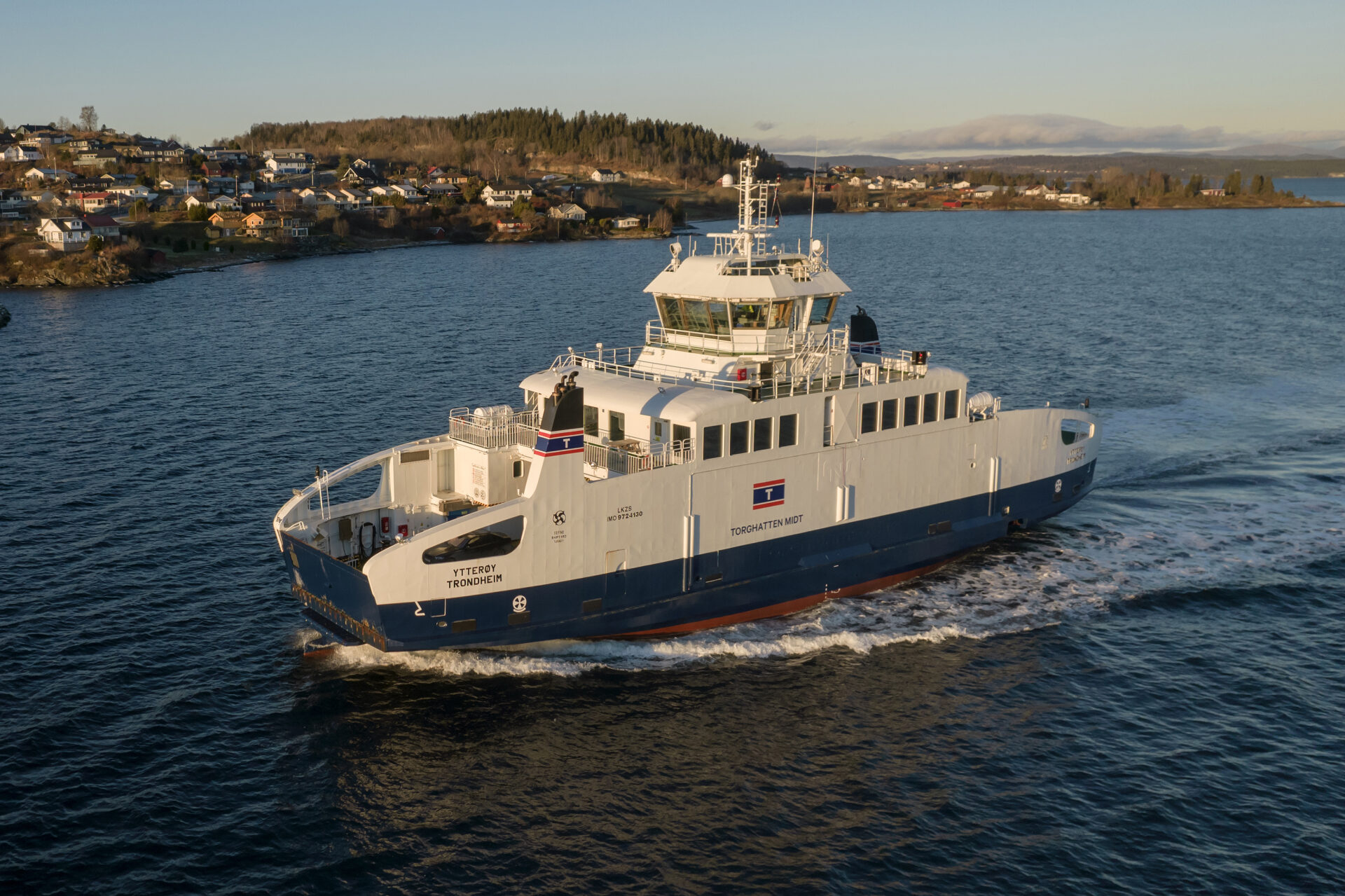
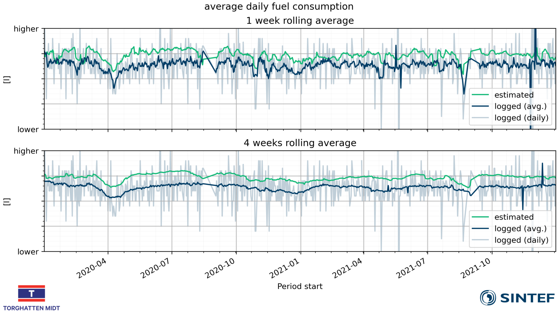
Case study: Ferry In connection with work taking place in SFI Autoship, the method described above has been used to estimate the consumption of MF Ytterøy (construction year 2015, 49.9 m long, 13.2 m wide, capacity of 38 PBE). The ferry serves the Levanger-Hokstad connection at the head of the Trondheim Fjord and is owned by Torghatten. In addition to open AIS data (Norwegian Coastal Administration) and open meteorological and oceanographic data (Norwegian Meteorological Institute), the vessel’s estimated speed-power graph in calm water (from the designer) and various data sheets from suppliers (e.g. the main engines) are also used. The estimates have been compared with daily readings of the level in the ferry’s fuel tank and information about when and how much fuel has been filled. Over a period of 2 years, the margin of miscalculation for the estimated annual consumption is between 13% and 15%, and the calculation time for the result is just a few minutes on a standard computer. While it is certainly possible to achieve greater precision using other methods, they will require readily available input (e.g. 3D drawings of the hull) and/or much greater computing power (e.g. computing clusters with hundreds of cores). At the other end of the scale, an experienced operator will be able to derive an assumed average consumption using knowledge about the boat and weather conditions in the area. Our approach attempts to place itself between these two extremes and balance the need for accuracy with the desire for the simplest possible input to the calculations and quick answers. The method generates a varying estimate, which changes according to weather conditions and operations (see the figure below and note, for example, lower consumption in April 2020). Therefore, it is suitable for analysing variations in consumption over longer periods of time, for which a static estimate or a very computationally intensive method could not be used.
While the method will provide an estimate for each crossing, its strengths can really be seen when analysing consumption over time periods in the order of weeks. For individual days, the error at its worst is around 50%, for weekly consumption this figure is reduced to 25%, and for consumption over a 4-week period, it is mainly between 10 and 20%. The figure below shows average consumption over one and four weeks. It can be seen that the estimates (green line) follow fluctuations in real consumption (blue line) closely, and the error mainly consists of an offset. For a one-week rolling average, the correlation coefficient between estimate and real consumption is 0.52, while it rises to 0.9 if averaged over a four-week period.
When will this method provide good results? The most certain part of the information available is the vessel’s behaviour in still waters and how it operates (speed profile). Weather conditions can be very local and correction for waves in particular can be challenging. It is therefore an advantage if the ship operates in relatively protected waters. The challenge with the accuracy of weather data may at first glance seem quite large, but in practice is often less serious if one has data from a long enough period, since the errors will even themselves out. Have you, for example, underestimated wind resistance when there is a direct headwind? The same thing happens when estimating how much help you get from a tailwind. This is especially true for vessels that have a fixed area of operation and fairly regular sailings. One will then sail just as much with a headwind as with a tailwind. Scheduled vessels such as ferries or express boats are therefore particularly suitable, but also PSVs or SOVs etc.
The results on which this article is based have been produced in connection with SFI Autoship (https://www.ntnu.edu/sfi-autoship). Many thanks to Torghatten (https://torghatten.no/) for good collaboration and permission to publish some results from analyses carried out on their routes. Open AIS data are made available by the Norwegian Coastal Administration (https://www.kystverket.no), and meteorological and oceanographic data by the Norwegian Meteorological Institute (http://met.no).
1 https://www.regjeringen.no/no/aktuelt/historisk-beslutning-om-nullutslipp-for-internasjonal-skipsfart/id2989641/
2 Norwegian Shipowners’ Association, 2021
3 Von Baeyer, Hans Christian (2001). The Fermi Solution
0 comments on “Energy consumption in today’s shipping fleet – how to make good estimates when we don’t have measurements?”