Talking to your simulator: What we learned building JutulGPT

In a companion post, we described our own experiments across a wide range of tasks, from refactoring a half-million-line production codebase to building wildfire simulators from scratch in a single day. The pace of change is remarkable, and the capabilities are broader than most people expect.

One application that has been a goal for our group in the last one-and-a-half years is a natural-language interface to complex scientific simulators: the ability to interact with your simulator the way you would interact with a knowledgeable colleague who runs simulations on your behalf. Rather than learning complex graphical user interfaces or intricate configuration syntaxes and API details, you describe what you want in plain language. The system interprets your intent, sets up the model, runs it, and reports back. If something is unclear, it asks. If something goes wrong, it explains why and suggests how to proceed. Agentic AI provides exactly the right architectural foundation for this kind of interface. This post describes what we learned building one.

1. Setting up a simulation model: a different kind of challenge

One of the most impressive capabilities of modern agentic coding tools is their ability to devise meaningful tests on their own, reasoning about what correctness should look like for a given component and verifying their work against those self-constructed criteria. This works well for isolated components: a linear solver can be tested against known solutions and convergence rates, a discretization scheme against patch tests and analytical benchmarks, an algebraic multigrid implementation against a reference solver. In each case, correctness is well-defined and directly testable.

Many technical software systems, however, are assembled from many such components that must work correctly together. Physics-based simulators are a prominent example. These are software systems that solve partial differential equations (PDEs) governing continuous physical processes, such as fluid flow, heat transfer, structural deformation, or electrochemical reactions. They typically consist of a mesh or grid representing the physical domain, discrete equations approximating the underlying mathematics, and a simulator that handles time-stepping, linearization, linear solvers, and convergence control. Setting up such a simulator for a given problem requires specifying not just individual components but the relationships between them, including constitutive relations, boundary and initial conditions, source terms, and solver tolerances. All of these must be mutually consistent and physically meaningful. The same broad challenges apply to many other complex technical systems, though the specific vocabulary differs.

For such systems, a script or configuration that sets up a simulation can be executed without errors even if parameters are out of physically meaningful ranges, constitutive relationships are physically incompatible with each other, or the numerical discretization is inconsistent with the mathematical model. Execution success, in this general setting, is a necessary but far from sufficient condition for a meaningful result.

A simulation model is only correct, strictly speaking, if the mathematical model faithfully captures both the physical process of interest and the specific scenario the user wants to investigate, the numerical model correctly approximates the mathematical model, and the simulator correctly implements and solves the numerical model. Choosing the right physical process is necessary but not sufficient: the model must also be configured with the right constitutive assumptions, parameter values, and boundary conditions to answer the question being asked. A standard coding agent constructing a simulation configuration from a natural-language description faces all three levels at once. It can reason about code, but it cannot necessarily verify the alignment between the model it builds and the user’s scientific intent. A simulation can be syntactically valid, numerically convergent, and still answer the wrong question.

A simulation that passes the simulator’s internal checks is physically consistent. Whether it answers the right question is a different matter.

Production-grade simulators, whether industrial or scientific, typically address part of this challenge through many internal consistency checks: validation of input parameters, enforcement of physical constraints, monitoring of solver convergence, and detection of numerical anomalies during the simulation itself. When such a simulator runs to completion, the model has passed these checks. That is a meaningfully stronger statement than the absence of a runtime error, and it is what makes such a simulator a suitable arbiter for agent-generated configurations.

To investigate this in a concrete setting, we chose the Jutul simulation framework written in Julia as our experimental platform. Jutul is a free, open-source, modular framework for composable and fully differentiable simulation of systems governed by PDEs, developed at SINTEF and released under the permissive MIT license. Several domain-specific simulators are built on top of it: JutulDarcy for subsurface flow and reservoir simulation, Fimbul for geothermal applications, BattMo for electrochemical battery simulation, and Mocca for gas adsorption processes, among others. We focus here on reservoir simulation as our primary context, using JutulDarcy, while noting that the principles apply across the Jutul ecosystem and more broadly to similar simulator frameworks. The agent interface we built on top of this framework is called JutulGPT.

2. Building the agent: choices and lessons

We began building JutulGPT in the summer of 2025. The landscape of agentic AI tools has moved substantially since then. Tools like Claude Code existed but were considerably less mature and capable than they are today, and the underlying models were less capable of sustained autonomous multi-step reasoning. We built on LangChain with a Python wrapper around JutulDarcy, a practical choice at the time, though one we would likely revisit today. What has not changed is the core architecture and the motivation behind it.

The choice of JutulDarcy as the simulation backend was deliberate and has held up well. Three properties made it particularly suitable for agent-mediated interaction. First, the software has both a file-driven and a programmatic interface. In the latter, models are assembled in Julia code rather than specified in keyword-heavy input files, which means the agent can construct and modify configurations through code generation rather than file editing; this is the mode we used. Second, the framework exposes explicit type structures, well-typed constructor interfaces, and structured error messages. Using static linting, the agent can then catch API mismatches early before the full script is written and executed rather than discovering them through a failed run. This allows the agent to self-repair at the right level and at the right time, rather than producing silently incorrect configurations. Third, because JutulDarcy is open source and well-documented, retrieval can surface not just isolated function signatures but relationships between components and common usage patterns.

One practical lesson emerged clearly from the early experiments: iteration is essential. An initial one-shot approach, generating the full simulation script from a single query, produced poor results. The agent would either retrieve an existing example unmodified or hallucinate non-working code. Adding a linting step before execution, and allowing the agent to iterate on errors, dramatically improved quality. This is the kind of verify-and-repair loop that is now built into modern agentic coding tools. We developed much of the same machinery ourselves, but at the time with considerably more manual effort. The field has since converged independently on these mechanisms, which is some confirmation that the approach was sound.

Documentation quality turned out to matter more than we had expected. We found that individual docstrings and structured text documentation were more immediately useful to the agent than long end-to-end example scripts. With today’s larger context windows this gap is smaller, but the underlying principle likely still holds: granular, well-structured docstrings support precise API use, and informative error messages allow the agent to self-correct efficiently. For simulator developers, this is a practical takeaway that applies regardless of which agent framework is used: treating documentation and error messages as agent infrastructure, not just human-readable text, pays off.

3. The interpret–act–validate loop in practice

JutulGPT supports a natural range of interaction modes, from simple documentation queries to fully autonomous model construction. The following examples illustrate this progression, starting with the underlying loop architecture and working through increasingly complex modeling tasks.

The interpret–act–validate loop

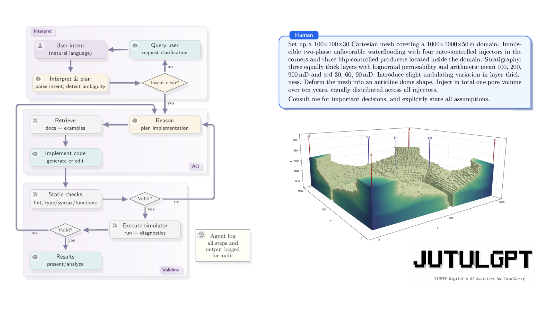
The architecture of JutulGPT organizes interaction with the simulator as an iterative loop with three phases, illustrated in Figure 1. In the interpret phase, the agent parses the user’s intent, identifies underspecified modeling choices, and either resolves ambiguities autonomously (with explicit logging of the assumption made) or escalates them to the user through targeted queries. In the act phase, the agent retrieves relevant documentation and examples, generates or modifies Julia code, and performs static analysis before execution. In the validate phase, the agent executes the code in a local Julia environment, analyzes solver diagnostics and runtime errors, and determines whether the result is physically and numerically admissible. If not, it revises and re-enters the loop. All steps, tool invocations, and outputs are logged throughout, providing a traceable record of the modeling process.

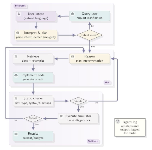
Figure 1. The interpret–act–validate loop used by JutulGPT. The agent incrementally interprets user intent, detects ambiguities, and resolves them either autonomously or via targeted user queries. Code generation is grounded in retrieved documentation and validated through static analysis and simulator execution. The loop terminates when the simulator runs to completion, which constitutes a validity certificate by virtue of JutulDarcy’s internal enforcement of conservation tolerances, closure consistency, and solver convergence.

Exploring documentation: a taxonomy of well models

At the simplest level, the agent can be asked to explore and summarize available functionality. Take the modeling of wells as an example. A reservoir simulation model consists of a spatial discretization of the subsurface with associated rock properties such as permeability and porosity, a fluid description, and a description of the wells through which fluids enter or leave the reservoir. The wells are the only physical connection between the simulator and the real world. Fluid flow and pressure communication through the well can be represented either by a semi-analytical model, which captures the essential flow behavior with a compact mathematical expression, or by a more complex discretized numerical flow model that resolves the wellbore in greater detail. Knowing what options are available in a given simulator, and how they relate to each other, is a prerequisite for setting up a physically meaningful model. The query we posed to JutulGPT was simply: “What kind of well models can I use in the simulator?” Figure 2 shows the response.

This mode does not involve any simulation, but it illustrates the agent’s ability to navigate a large, distributed codebase and surface relationships that are not apparent from isolated docstrings.

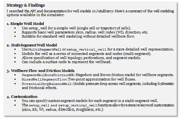
Figure 2. JutulGPT response to the query “What kind of well models can I use in the simulator?” The agent searched documentation and source code and synthesized the results into a structured taxonomy, surfacing relationships between model types and typical usage scenarios.

A central question in improved hydrocarbon recovery is how efficiently an injected fluid sweeps through the porous rock and displaces the hydrocarbons one wants to produce. Injection is typically used both to maintain reservoir pressure, which pushes fluids to the surface and would otherwise decline as fluids are produced, and to physically displace oil or gas toward the production wells. How well this displacement works (i.e., how much of the reservoir is contacted and swept by the injected fluid) directly determines how much can be recovered. The quarter five-spot is the canonical benchmark for studying displacement efficiency: a single injector and a single producer placed at opposite corners of a square domain, designed to isolate this effect in a controlled, symmetric setting.

In a two-phase scenario, the interesting parameter is the mobility ratio M between the injected and displaced fluid. When M < 1 (favorable displacement), the injected fluid is less mobile and the displacement front remains relatively stable, giving good displacement efficiency. When M > 1 (unfavorable displacement), the injected fluid is more mobile and tends to channel through the reservoir, reaching the producer early while leaving much of the domain unswept.

We asked the agent to set up two such simulations contrasting the two regimes, specifying only the physical objective and asking it to request clarification if anything was missing (see the prompt in Figure 3). The prompt does not specify how to implement the difference between favorable and unfavorable displacement. The agent reasons correctly that the distinction is realized through the viscosity ratio between the two fluids, selects appropriate values, and produces two comparable simulations that isolate precisely the effect the user wants to illustrate. It parsed the intent, retrieved relevant examples, generated code, encountered a constructor mismatch where keyword arguments were used where positional arguments were required, self-repaired in one cycle, and autonomously delivered two validated simulation setups in less than a minute.

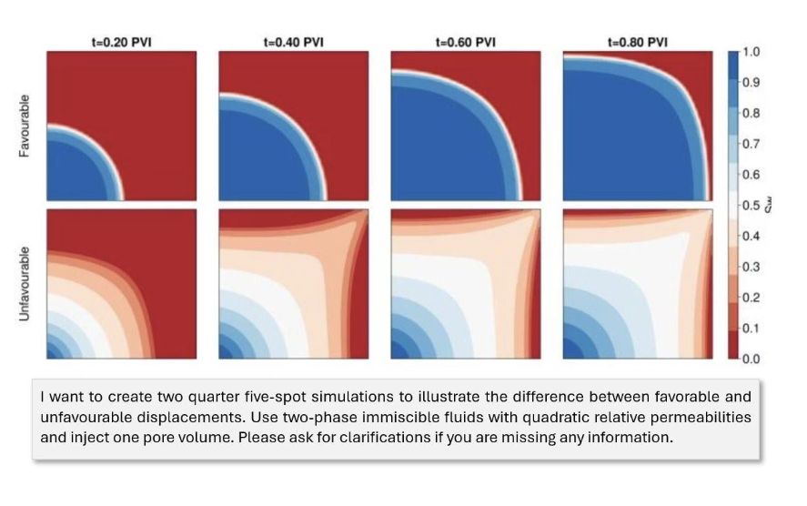
Figure 3. JutulGPT output for the quarter five-spot displacement example. The user prompt is shown in the box below the results. Saturation fields at four time steps (0.20, 0.40, 0.60 and 0.80 pore volumes injected) are shown for the favorable case (top row) and unfavorable case (bottom row).

A heterogeneous 3D reservoir model

The quarter five-spot is a textbook problem, useful for isolating specific physical effects but far from the complexity of real field applications. To test JutulGPT on more demanding cases, we moved to semi-realistic synthetic models: configurations that capture some structural and petrophysical complexity, but without the large volumes of geological, geophysical, and petrophysical data that a real field study would require. One set of experiments involved reservoirs with explicitly modeled fractures: ellipsoidal in shape, with permeability that tapers toward the fracture tips in accordance with standard models from linear elastic fracture mechanics. The results were, from our perspective as non-specialists in reservoir characterization, surprisingly good. We present a simpler example here, but the intent is to give a sense that these are not toy cases.

The example in Figure 4 was chosen specifically because it required the agent to set up a non-rectangular geometry and find and correctly apply geostatistical methods for assigning heterogeneous rock properties. Generating physically meaningful lognormal permeability fields layer by layer, with the right statistical parameters and sampling strategy, is not something one can do by guessing at API calls in JutulDarcy.

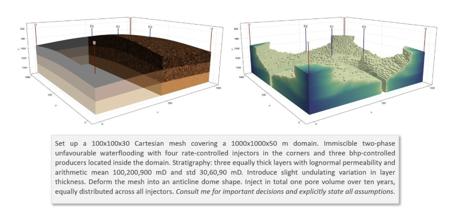
Figure 4. JutulGPT output for the heterogeneous anticline scenario, run in interactive mode. The agent consulted the user for consequential decisions and logged all assumptions explicitly. The left panel shows the smooth layered anticline; the right panel shows water saturation after the injected water has reached the producers.

Rather than generating code immediately, the agent entered a structured clarification phase. It identified the underspecified choices that would materially affect the model: porosity specification, fluid viscosities, relative permeability parameters, well coordinates, and deformation amplitudes. For each, it proposed an explicit default with physical justification and requested confirmation. One user override was incorporated, replacing constant porosity with a lognormal distribution. The agent then assembled the full model: deforming the grid into the anticline shape, assigning geostatistical property distributions layer by layer, placing injectors and producers, computing the total pore volume of the deformed grid, and deriving injection rates to ensure that exactly one pore volume would be injected over ten years, equally distributed among the four injectors. The loop terminated only after successful completion of the full ten-year simulation on the 300,000-cell grid, with verified satisfaction of the global injection target.

When the agent showed it understood

Two moments from our experiments illustrated that the agent was doing more than pattern-matching on code. In the first, a colleague constructed a prompt for a standard setup, but with a domain so small that the well cells were narrower than the well diameter itself; a subtle physical inconsistency that would cause an error. The agent caught the problem, explained precisely why it occurred, and suggested how to fix it. The issue is a classic one: anyone who has supervised students in reservoir simulation will have seen exactly this mistake.

In the second, a colleague asked the agent to convert an existing simulation script to run in parallel using MPI (Message Passing Interface), the standard framework for distributed-memory parallelism where computation is spread across multiple machines, each with its own memory — as opposed to parallelism within a single node. This is considerably more complex to set up correctly. The request was their very first experiment with the agent. It read the parallelism documentation, set up the required packages, modified the script in exactly the right places, and provided a shell script to launch the job with the correct number of MPI processes. The result worked on the first attempt.

4. Trust and reproducibility

For an agent to be genuinely useful in scientific work, it must do more than produce results. It must be possible to inspect, question, and audit what it did. The expectation is not so different from what one would have of a graduate student or a scientific assistant: a brief account of what was done, what choices were made and why, and enough traceability that a supervisor can follow up on anything that looks unexpected.

Auditing what the agent did

We were therefore careful to build comprehensive logging into JutulGPT from the start. Every resolved ambiguity, every retrieved document, every assumption and tool invocation is recorded. But a raw execution log is not always easy to read, and auditability also requires that the agent can summarize what it did at different levels of abstraction, the way one might write a brief Slack message, a slide deck, or a formal report depending on the audience and purpose.

With this in mind, we asked the agent to produce three such representations after completing the 3D anticline model: a detailed reproduction prompt intended to recreate the model exactly, a formal technical report with governing equations expressed in simulator-agnostic terms, and a compact description of the kind one might include in a journal paper. These three artifacts encode the same physical scenario at progressively increasing levels of abstraction, and they gave us a concrete basis for asking a further question: how much of the simulation is captured by each representation?

Testing reproducibility

Anyone who has attempted to reproduce a published simulation from a textual description knows that it is harder than it looks. Natural-language descriptions are inherently underspecified: they may omit details the author considered obvious, leave physical parameters implicit, or fail to distinguish between modeling choices that are mathematically equivalent but computationally distinct. Different modelers reading the same description will make different admissible choices, and the resulting simulations may diverge in ways that are difficult to diagnose after the fact.

We had this in mind partly because of our own experience organizing the 11th SPE Comparative Solution Project for geological CO₂ storage; a community benchmarking exercise in which research groups and companies independently simulate the same problem and compare results to assess state-of-the-art in simulation technology and pinpoint needs for future research. The study aimed for a fully specified mathematical model, yet intercomparison of results from 18 contributing teams revealed substantial variation, driven not only by different interpretations of the problem description but also by implementation choices the description could not fully constrain. A detailed specification, it turned out, is not the same as a uniquely determined computational experiment.

We initialized three independent agents, each given only one of the three representations and no access to the original code, and asked them to reconstruct an executable simulation. All three succeeded in producing simulations that ran correctly and generated physically plausible results. But they differed from the reference in instructive ways.

The tacit-assumption gap

In building the reference model, the agent had utilized a density-model constructor whose default behavior was to apply a compressible fluid formulation. This was never an explicit decision: the agent simply invoked the constructor, the default was applied silently, and the choice was never logged. Because it was never logged, it did not appear in any of the three textual representations derived from the model.

The assumption log records what the agent decided. It does not record what the agent inherited.

When the three autonomous reconstruction agents encountered this unspecified parameter, each resolved it independently. The technical report and journal-style reconstructions both set compressibility to zero, producing incompressible models; the reproduction prompt reconstruction arrived at a compressible formulation, matching the reference. None of these outcomes was predetermined: each agent made a reasonable choice given what the representation told it, and the representation told it nothing about compressibility. This randomness, inherent to autonomous agents operating without human guidance on unspecified parameters, is what makes the gap structural rather than incidental.

The difference in physical behavior was substantial, as shown in Figure 5. In the compressible reference case, higher oil compressibility reduces the effective density contrast and weakens buoyancy, allowing viscous fingering to produce a mixed, complex saturation pattern. In the incompressible reconstructions, the full density contrast drives rapid buoyancy segregation, with denser water underriding lighter oil and channeling along the high-permeability bottom layer. These are genuinely different physical behaviors, not a minor numerical deviation.

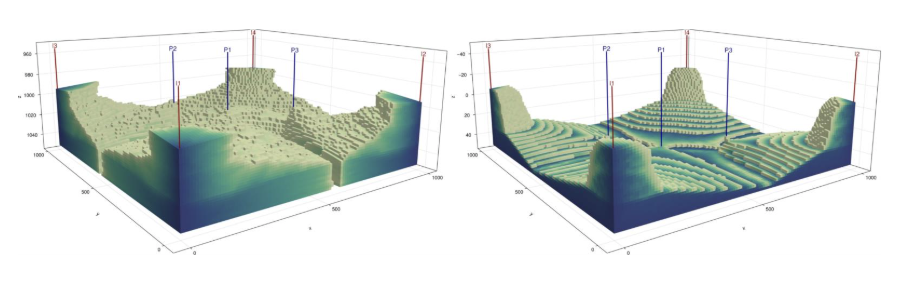
Figure 5. The heterogeneous anticline model rendered with permeability coloring. Left: the compressible reference model. Right: the incompressible reconstruction from the technical report. The difference in fluid compressibility, never explicitly specified and therefore absent from all three textual representations — produces qualitatively different flow behavior.

The journal-style description, as one would expect from its level of abstraction, produced additional differences beyond compressibility: reinterpretation of well placement into a symmetric configuration, and reconstruction of the dome geometry using different functional forms. These too are admissible interpretations within the degrees of freedom left open by the representation. Reconstruction variability, in this sense, makes implicit modeling choices visible; it is a practical tool for auditing what a simulation description actually determines, and what it leaves open.

Reliable reproduction requires the executable state: the generated code together with pinned simulator versions and dependencies. The agent’s construction log is a necessary complement, but it cannot surface choices that were never part of the agent’s assumption space. Closing that gap requires deliberate co-design of agents and simulators.

5. Practical implications: designing simulators for agent access

Building an effective agentic interface to a simulator is not primarily a matter of adding an API layer. The more fundamental question is what properties of the simulator make it work well with an agent in the first place.

JutulDarcy has several such properties that worked in our favor. Explicit type structures and typed constructor interfaces mean that API mismatches produce informative, targeted errors rather than silent wrong behavior. Structured solver diagnostics like convergence failures, timestep reductions, and conservation errors give the agent precise signals to act on rather than opaque failure states. Open-source, indexed documentation allows retrieval to surface semantic relationships between components, not just isolated function signatures.

The tacit-assumption gap points to a further design direction: simulators should, where possible, make their defaults explicit and auditable. A constructor that silently applies a compressible density model should ideally log that choice in a form the agent can inspect. This can be done, but only if simulator developers make it an explicit goal; it will not emerge on its own.

A complementary direction is to expose simulator functionality through standardized tool interfaces such as the Model Context Protocol (MCP), allowing general-purpose agents to interact with domain-specific simulation capabilities without requiring a fully custom implementation. This lowers the barrier to building simulator-specific agents and makes the interface maintainable as both the agent ecosystem and the simulator evolve.

6. Looking ahead

We began this work in June 2025. The agentic AI landscape has moved substantially since then, and it is worth being candid about what that means for the technical choices we made and the conclusions we drew.

The software stack (LangChain, locally hosted models, a Python wrapper around Julia) made sense at the time; today we would likely take a different approach, building on tools like Claude Code and exposing JutulDarcy as an MCP server rather than wrapping it in a custom Python interface. The loop architecture and the motivation for embedding the agent inside the simulator remain as valid as ever. The specific capability observations — that agents can iterate on errors, read documentation, and modify code surgically — are now broadly understood. What has not changed, and what we believe will remain relevant for some time, is the tacit-assumption gap. It is not a limitation of any particular model or tool; it is a structural property of the interface between natural-language descriptions and executable simulator state. Better agents will make fewer explicit mistakes. They will not automatically make fewer tacit ones. The same applies to the practical lessons about documentation granularity and error message quality: these are properties of the simulator, not the agent, and improving them benefits human users and agent-mediated workflows alike.

Better agents will make fewer explicit mistakes. They will not automatically make fewer tacit ones.

What the current system does not yet do is at least as interesting as what it does. JutulGPT sets up and runs simulations; it does not visualize or present results in a form suited to the user’s question. It does not interpret what the simulation reveals, reason about whether the outcome is physically sensible, or suggest what to do next. It cannot close the loop back to model refinement when results fall short. It does not connect to observational data for history matching, does not systematically explore parameter space for uncertainty quantification, and does not optimize model parameters against a target. Each of these is a natural next step, and taken together, they describe the kind of agent that would genuinely function as a scientific colleague rather than a sophisticated setup tool: that is the system we are working toward.

Paper and code

Paper, code, prompts, and agent logs: arXiv:2603.00214
JutulGPT source code: github.com/SINTEF-agentlab/JutulGPT